Excel VLOOKUP Function
The VLOOKUP Function (which stands for "vertical lookup") is one of the most useful functions in Excel, and is a fast way to look up a value when your information is arranged in a table with rows and columns. The VLOOKUP function has four arguments (values in the function separated by commas) and because of this people often think VLOOKUP is complex. Once you try a few practice problems with VLOOKUP you'll see how simple it really is.
Syntax of the VLOOKUP Function
If your data is arranged in a table with rows and columns, the VLOOKUP function will tell you a value in one row if you know a different, corresponding value to the left in that same row (the VLOOKUP function only looks from left to right). For the VLOOKUP example below, say you have a table with columns for employee ID, hire date, and employee name in your Excel spreadsheet, as shown in the image below. Each row represents a different employee. Say you want to retrieve the name of the employee with ID 1234 using VLOOKUP.
=VLOOKUP(lookup_value, lookup_range, column_number, [approximate_match])
- Lookup_value: This is the value that you know, which you will use to locate the value that you do not know. In this example it is the employee ID, which is 1234
- Lookup_range: This is the entire table, also called the lookup table or table array, that we are searching. We could say A1:C6. If this was a long list we could use the entire columns A:C
- Column_number: The columns in your lookup_range table are numbered from left to right, starting with 1. The VLOOKUP function will locate the lookup_value in column 1 (far left) and return the value in the same row but in the column specified by column_number. The employee ID column is 1, the hire date column is 2, and the employee name column is 3. Note that VLOOKUP only searches from left (starting in column 1) to right. Because we want VLOOKUP to return the employee's name, we will specify 3 for column_number.
- Approximate_match: This is the only optional argument, though it's recommended that you specify it as false (it defaults to true) when you know the lookup_value. In our case we can say false or 0; we want an exact match on 1234. The default value is true, so if you leave this blank Excel will tell VLOOKUP will look for approximate matches, which we typically don't want except for special cases.
So, in order to use the VLOOKUP function in Excel to find the name of the employee whose ID is 1234, you could use the formula =VLOOKUP(1234, A1:C6, 3, false). See image below for details.
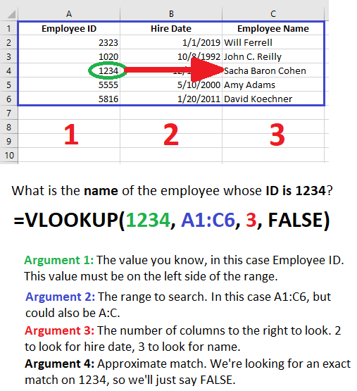
Note that the value you know (the first argument) must always be in the first column (on the far left side) of the range you choose.
VLOOKUP Practice Exercises
Suppose we are tracking employee names and information in Excel, but our columns are now in a different order with Employee name, employee ID, and hire date in the first column, second column, and third column, respectively. The following are VLOOKUP examples with the new, rearranged lookup table.
| A | B | C | |
|---|---|---|---|
| 1 | Employee Name | Employee ID | Hire Date |
| 2 | Will Ferrell | 2323 | 1/1/2019 |
| 3 | John C. Reilly | 1020 | 10/8/1992 |
| 4 | Sacha Baron Cohen | 1234 | 12/10/2005 |
| 5 | Amy Adams | 5555 | 5/10/2000 |
| 6 | David Koechner | 5816 | 1/20/2011 |
Use VLOOKUP to Find Will's Employee ID
The value we know in the first column is "Will Ferrell" and our lookup range can be A:B, A:C, or A1:B6, etc. Employee name is column 1 in our lookup range, and we want Employee ID so we will specify 2 for column number. Finally, we know exactly how to spell our lookup_value (Will Ferrell) so we will specify false for approximate_match.
=VLOOKUP("Will Ferrell", A:B, 2, false)
This VLOOKUP formula will return the value 2323, which is in column 2 of our table array in the same row as the lookup value.
Use VLOOKUP to Find the Hire Date of the Employee With ID 1234
This example is a little trickier because Employee ID will be our lookup value instead of Employee Name. Recall that the lookup value needs to be in the first column of our lookup table, so we will need to specify B:C or B1:C6 as our lookup range.
=VLOOKUP(1234, B:C, 2, false)
This VLOOKUP formula will search column B from the top down until it finds 1234, then will look in column 2 (column C) of the lookup table in the same row to return a value of 12/10/2005.
VLOOKUP With Wildcard Matching
Excel lets you use the VLOOKUP function with wildcards. Note that this only works in exact matching mode, so your fourth argument (approximate_match) must be 0 or FALSE. Remember, you can't omit this argument because Excel defaults approximate_match to true. Also note that this only works for matching strings of text.
What is Wildcard Matching in Excel?
Wildcard matching in Excel is the ability to use characters which represent anything in a string of text. For example, say you know someone's first name but not their last name. You could find this person in an Excel spreadsheet by concatenating their first name with a wildcard character.
A question mark (?) replaces exactly one character in a string of text in Excel.
An asterisk (*) replaces any number of characters in a string of text in Excel.
To use a wildcard in Excel, you concatenate an asterisk enclosed in quotes at the beginning or end (or both) of your string of text. It looks like this:
=VLOOKUP("My text"&"*", A:C, 2, FALSE)
The VLOOKUP function will then return the first value it finds where the lookup_value is text that begins with "My text". If our lookup_value was instead "*"&"my text", then it would search for any text that ends with "my text" because the asterisk comes first.
| A | B | C | |
|---|---|---|---|
| 1 | Employee Name | Employee ID | Hire Date |
| 2 | Will Ferrell | 2323 | 1/1/2019 |
| 3 | John C. Reilly | 1020 | 10/8/1992 |
| 4 | Sacha Baron Cohen | 1234 | 12/10/2005 |
| 5 | Amy Adams | 5555 | 5/10/2000 |
| 6 | David Koechner | 5816 | 1/20/2011 |
Say we want to find the ID number of the employee whose first name is "Amy". We could use the wildcard match as follows:
=VLOOKUP("Amy"&"*", A:B, 2, FALSE)
This will return the ID number of the first employee in the table whose name starts with the text "Amy". Now suppose you want to find the ID of the employee whose middle initial is C. You can use wildcard at the beginning and end of the search string as follows:
=VLOOKUP("*"&"C."&"*", A:B, 2, FALSE)
This will return the ID of the first employee who has "C." in their name.
Exact Match vs. Approximate Match
Excel lets you use VLOOKUP to search for an exact match or an approximate match, as determined by the fourth argument, which is optional. VLOOKUP defaults to approximate match, so if you omit the fourth argument, or if you include it as TRUE or 1, then VLOOKUP will use an approximate match.
If you include the fourth argument as 0 or FALSE, then VLOOKUP will use an exact match.
Exact matching makes sense when you're searching for an exact value, like Employee ID number in the examples above. If you don't match on the exact ID number, you may get the wrong employee!
If you're not sure whether the exact value appears in the list, you can use approximate match to find the value that matches best. If Excel does find an exact match, then it will match on that value. If it does not find an exact match, it will find the closest value to match.
If VLOOKUP is using an approximate match it will use an exact match if the exact value is available. If not, it will use the next smallest value, so if you're using an approximate match in Excel you need to make sure the first column is sorted from small to large, or alphabetically.
VLOOKUP Errors
The VLOOKUP function in Excel is prone to errors because it has so many required arguments, and if any part of the formula is written incorrectly it will result in an error. Unfortunately, the error messages that Excel provides are not very helpful in diagnosing the problem. Read on to learn more about the different error messages you might see while writing a VLOOKUP formula in Excel and how to correct them.
VLOOKUP Function is Returning the #N/A! Error
The VLOOKUP function returns the #N/A! error when it is looking for an exact match (approximate_match is false) and it cannot locate the lookup_value. To fix this error, ensure that the lookup_value is spelled correctly in both the formula and the lookup table, and double check the defined lookup_range. Ensure that the lookup_value is in the left-most column of the lookup_range. Also ensure that the lookup_value is the same format in both the formula and in the lookup table; if a number is formatted as text in one of these places the VLOOKUP function will not consider them a match.
VLOOKUP Function is Returning the #REF! Error
The VLOOKUP function in Excel returns the #REF! error if the formula references a column that is not included in the lookup_range. To fix this issue, double check the lookup_range and count the number of columns included in the lookup table. Then double check the column_number argument (the 3rd argument of a VLOOKUP formula) and ensure that the number is not greater than the total number of columns in the lookup table. The column_number argument can be any number from 1 to the total number of columns in the lookup table.
VLOOKUP Function is Returning the #VALUE! Error
The VLOOKUP function returns the #VALUE! error if the column_number or approximate_match arguments are invalid values. To fix this issue, first double check the column_number argument and ensure that it is a number (greater than 0) and is not text, a negative number, or anything else. Next, double check the approximate_match argument and ensure that it is either omitted or is a valid boolean (true or false) value. It must either be the words "true" or "false" (without the quotation marks). Alternatively, in Excel, boolean values can be 1 for true and 0 for false. Any other values will be considered invalid.
VLOOKUP Function is Returning a Value I Do Not Expect
Is the VLOOKUP function returning a value you're not expecting, and you're not sure why? We've all been there. The first thing to check is that the fourth and final argument is set to false, provided that you know the exact value of the lookup_value. If the approximate_match argument is true or if it is left out of the formula, it will default to true and VLOOKUP will look for an approximate match, which can cause all kinds of unexpected problems.
The second thing to check is whether there are multiple instances of the first argument (the lookup_value) in the first column of the lookup table. If the lookup_value is listed more than once, the VLOOKUP function will simply match with the first one that it finds, which is whichever row is highest in the lookup table since VLOOKUP in Excel searches from top to bottom. So if VLOOKUP is returning an unexpected result but from the correct column, make sure that the lookup_value doesn't appear again higher up in the lookup table.
While you're checking for a second instance of the lookup_value, also note that when VLOOKUP matches with the lookup_value, it is NOT case sensitive. This means that, to the VLOOKUP function in Excel, "robert de niro" is the same as "Robert De Niro" amd will treat them the same. So when you're checking that the lookup_value only exists once in the table, also check for the same value with different capitalization.